
BestCurvFit software at an affordable price
New Improved Version 14.1 (May 1, 2025)
BestCurvFit performs nonlinear regression curve-fitting of data to kinetic models either defined by the user or selected from in internal library of 46 models. BestCurvFit is priced to make it affordable to professionals and students alike. But don't let the low price mislead you. BestCurvFit is robust and powerful using some of the most sophisticated regression algorithms, including Variable Metric, Gauss-Newton as modified by Marquardt-Levenberg , Conjugate Gradient, Hooke-Reeves, and Random search methods. Why pay hundreds and yearly license fees when you can have curve-fitting software for a fraction of the cost. Best of all, there are no time limit restrictions or number of uses.
With just one-click of the mouse, BestCurvFit simplifies curve fitting your data to mathematical models. Select an equation from an internal library of 46 models or enter your own function, and BestCurvFit does the rest by fitting the curve to your data set, displaying the statistical results, model parameters, the best fit curve, and the residuals.
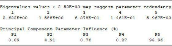
The BestCurvFit results of your curve-fit includes the fitted parameters, their standard errors, their significance , confidence limits, correlation matrix, and measures of parameter redundancy like variance decomposition proportions and condition index analyses, and eigenvalues and principle component values.
An important measure of a good curve-fit is the residuals plot. BestCurvFIt includes statistic tests for the residuals plot. These tests include (1) Distribution-free Runs statistic test of the randomness of residuals, (2) F-test statistic to determine if the mean of the residuals is significantly different than zero, (3) Durbin-Watson statistic test of residuals to determine if a serial correlation exists, (4) Kolmogorov-Smirnov non-parametric, distribution-free, statistic test of residuals to determine whether positive and negative residuals come from the same distribution, (5) Hotelling's T-squared distribution (T²) multivariate statistic used to measure dissimilarity for outlier detection in the data set, and (6) Besseli0 function of residuals to detect outlying data.
Multicollinearity of Regression Variables
When performing nonlinear regression of data to mathematical models, some explanatory variables may be intercorrelated and produce significant effects on each another. This relationship can compromise the results of multivariable regression analyses. The intercorrelation between explanatory variables is called “multicollinearity.” Multicollinearity represents a high degree of linear intercorrelation between explanatory variables in a regression model and may lead to incorrect results of the regression analyses. The condition index and variance decomposition proportion (VDP) can be used as a diagnostic tool to detect multicollinearity. Eigenvectors derived from eigenvalues are used to calculate the VDPs, and represent the extent of variance inflation by multicollinearity. This allows the determination of the variables involved in the multicollinearity. Each explanatory variable has VDP corresponding to each condition index. When two or more VDPs, which correspond to a common condition index higher than 30, are higher than 0.30, their associated explanatory variables are considered multicollinear and indicate near-linear dependence. Multicollinearity can inflate the variances of the explanatory variables, making the coefficients statistically insignificant and widen their confidence intervals. Excluding or masking multicollinear explanatory variables is a way to improve the stability of regression models. BestCurvFit uses the condition index and VDP to detect multicollinearity of explanatory variables in its results.
Price (Dollars $) Range ($)
PayPal or Credit card $29.99 - $49.99
Go to our Software page to download and purchase BestCurvFit using PayPal (VISA, MasterCard, Discover, American Express). PayPal uses the latest technology and proprietary procedures to protect the security of its transactions. PayPal automatically encrypts your confidential information in transit from your computer to theirs.
Other available software...

BestCurvFit - Nonlinear Regression Curve-fitting Software
There are several good reasons why BestCurvFit is a good choice for analyzing models to experimental data. It's one of the best, easiest to use, and most economical and robust MS Windows software for curve-fitting analysis. Just enter your data and model function in a text file, open the file in the software, and one click of the mouse produces curve-fit statistical results to determine the best-fit model. Instant graphs of data including X-Y, Hanes-Woolf, Semi-log, and Residual plots are available at the click of a button.
BestCurvFit software for MS Windows uses nonlinear regression to curve-fit data to the chosen mathematical model. Nonlinear regression is an iterative process of adjusting the model parameters until the chosen model best fits the data. Just enter the data and model in a text file, open the file in the software, and one click of the mouse produces curve-fitting statistics to determine the best-fit model. The program adjusts the model parameters so that the model curve comes as close as possible to the data points. When no further improvement in the fit can be made, the program stops and reports the best-fit results and statistics of the analysis. Graphs are display instantly by selecting the appropriate plot type - X versus Y, Hanes-Woolf X/Y versus X, Semi-log(X) versus Y, and Residual Y plot. A library of 46 kinetic models is included to facilitate the analysis of enzyme kinetic data, or you can create your own custom User-Defined-Functions (UDF) for curve-fitting. A UDF can have up to 8 parameters P1..P8 and 3 independent X1..X3 variables. BestCurvFit saves the results of each analysis in a text file with the data file name. It also creates a cummulative dated log file of all analyses which you should delete if it becomes too large. Installation is easy, BestCurvfit does not require MS Windows installation; just save the executable, *.ini, and *lic files to a folder. BestCurvFit is a stand alone executable program with no dynamic link library files (DLL's).
BestCurvFit Accuracy
The Statistical Reference Datasets (StRD) Project of the National Institute of Standards and Technology (NIST) has created a set of challenging nonlinear regression problems used to test nonlinear regression algorithms. NIST states that "a good nonlinear least squares procedure should be able to duplicate the certified results to at least 4 or 5 digits". BestCurvFit analyses of 22 NIST datasets produced an average accuracy of 6 decimal places using numerical derivatives.
- Average Number of Digits Achieved by BestCurvFit: 6.0
See the FAQ page for further details.
BestCurvFit Software running under MS Windows
The BestCurvFit software is copy protected to run on one MS Windows computer only. One additional license is allowed upon request as a backup if your computer is replaced. Simply download the software, unzip it, and run BestCurvFit on the computer you want to license it on and email us ( DrFrank88@gmail.com ) the displayed "Registration Code" after you purchase the software, and we'll send you the software license "Activation Code" to enter in the software and activate a fully functional copy. There are no time limits or number of uses once the software is activated.
See the Software page for further details.
Reaction scheme of the General Modifier Mechanism
of Botts and Morales
This scheme is based on the rapid-equilibrium assumption and describes the basic mechanism for the all classical reversible inhibition mechanisms. At saturating inhibitor concentrations the enzyme activity is either fully or partially inhibited depending on the value of 'b' (beta). The inhibition response can be either linear (b = 0) or partial and hyperbolic (0 < b < 1). In other words, at saturating inhibitor concentrations the remaining enzyme activity is either fully or partially decreased, respectively. If b = 1 then both ES and ESI are equally catalytically activity. In contrast, when b = 0 then only the ES complex forms product. The factor 'a' (alpha) represents the difference in binding affinities between the substrate binding to the EI complex and the inhibitor binding to the ES complex. When a = 1 the binding is equal, but when a = 0, only the inhibitor binds to the free enzyme. Differing values of 'a' and 'b' can be used to obtain all the common types of inhibition models. Competitive, uncompetitive, noncompetitive, or mixed type inhibition can generally be distinguished by the values of 'a' and Ki. See the 'Enzyme_Kinetics' web page of this site for an explanation of IC50 values using 'a' to determine the linear inhibition type.
Scheme and Equation for the General Modifier Mechanism
E: enzyme, ES: enzyme-substrate complex, ESI: enzyme-substrate-inhibitor complex, S: substrate, I: inhibitor, P: product of reaction, Km: substrate dissociation constant, Ki: inhibitor binding dissociation constant, kcat: catalytic rate constant, and 'a' and 'b' are dimensionless constants that define the type of the inhibition mechanism.
See link to Antonio Baici's Website "Kinetics of Enzyme-Modifier Interactions" below:


BestCurvFit Model #37 analysis: Km=86.2, Vmax=50.2, Ki=40.1, a=2.2, b=0.37

BestCurvFit Model #37 analysis:See "The Final Polish" at https://www.enzyme-modifier.ch/the-final-polish/
See link to the 'Enzyme_Kinetics' Webpage below for an explanation of IC50 formulas using the alpha value of Linear Mixed inhibition models.
Example of Yonetani-Theorell model
Yonetani-Theorell method of exclusivity of inhibitor interactions with an enzyme involves measuring the initial velocity of the enzyme at different concentrations of two inhibitors. The effects of the two inhibitors on the velocity of the enzymatic reaction can be described by the relationship, vi= Vo/(1 + I/Ki + J/Kj + (I*J)/(alpha*Ki*Kj)) where vi is the initial velocity in the presence of both inhibitors, Ki and Kj are the dissociation constants for inhibitors I and J, respectively, and alpha is an interaction term that defines the effect of the binding of one inhibitor on the affinity of the second inhibitor.
BestCurvFit plot of Yonetani-Theorell analysis

BestCurvFit Model #21 Analysis
Example of Mixed Noncompetitive Inhibition
Mixed type inhibition is similar to noncompetitive inhibition except that the binding of the substrate or inhibitor to the enzyme affects the binding of the other. In noncompetitive inhibition the inhibitor binds to a part of the enzyme or enzyme–substrate complex other than the active site. This deforms the active site so that the enzyme cannot catalyse the normal reaction.

Model #7 Mixed inhibition of enzyme activity

Results of Mixed inhibition analysis
Example of Five-Parameter Logistic model
BestCurvFit nonlinear regression analysis results and graphs

BestCurvFit Model #23 Main Menu

Semilog Dose-response of 5p-Logistic Model

BestCurvFit Results
Example of Global Michaelis-Menten
Curve-Fit of Enzyme Kinetic Data
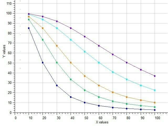
The simultaneous fitting of functions to multiple data sets with shared parameters is considered a global curve-fit. An example of a global curve-fit is the nonlinear regression analysis of multiple Michaelis-Menten functions containing a global Km parameter and multiple local Vmax parameters. Parameters that are estimated from all data sets are considered global, and those that are estimated from single data sets among multiple data sets are local. A global analysis is performed when a practicioner wants to combine all data from multiple experiments to determine a single global Km value of the Michaelis-Menten function even though the Vmax values differ among data sets.
For example, five separate data sets can be analyzed using five Vmax parameters but only one global Km parameter in a model containing five Michaelis-Menten functions. BestCurvFit performs this global curve-fit using a second independent variable X2 as an index variable to identify the separate data sets and functions. The data with the substrate (X1) are in column one, the index variable (X2) is in column 2, and rate data is in column 3. The index variable X2 is used to associate each of the functions with the corresponding data set. The User-defined (UDF) model for a global fit of the Michaelis-Menten function to five data sets is shown below. This is an example and the user can create their own UDF to fit their specific need.
Y = P2*(X2=1)/(1.0+P1/X1) + P3*(X2=2)/(1.0+P1/X1) + P4*(X2=3)/(1.0+P1/X1) + P5*(X2=4)/(1.0+P1/X1) + P6*(X2=5)/(1.0+P1/X1)
where the P1 parameter represents the global Km and the P2...P6 parameters represent the multiple local Vmax values.
The index variable X2 is represented in a logical function. For example, when the index X2 equals 1 (e.g., (X2=1)), the first data set is evaluated, otherwise it is false giving a value of zero.
The BestCurvFit analysis of the Michaelis-Menten model to five data sets is shown in the following graph. A good representative curve-fit was obtained providing a global Km value near 20. Reference: Duggleby, R.G. Pooling and Comparing Estimates from Several Experiments of a Michaelis Constant for an Enzyme, Anal. Biochem. 189 (1990), 84-87.

BestCurvFit analysis of five Michaelis-Menten functions in a single model.
Example of Gaddum-Schild Model
The Gaddum-Schild model #41 is used to determine the potency of competitive antagonists to their agonist receptor binding sites. When an antagonist (competitive inhibitor) competes for agonist binding to its receptor, the dose-response curve shifts to the right. The affinity of the competitive inhibitor can be determine by curve-fitting multiple curves each using higher concentrations of antagonist (inhibitor). The Gaddum-Schild equation is based on the assumptions that agonist and antagonist combine with the receptor macromolecule in a freely reversible but mutually exclusive manner.
Logistic-Gaddum-Schild model :
Independent variables:
X1 = Log10[agonist] molar
X2 = [antagonist] molar
Dependent variable:
Y = response of dependent variable
Model Parameters to optimize:
P1 = Log10(EC50) molar
P2 = pA2, where Kb=dissociation equilibrium constant, Kb = 10^(-pA2) = 10^-(-Log10(antagonist))
P3 = Minimum response plateau
P4 = Maximum response plateau
P5 = Hill slope of the response curve (positive for ascending and negative for descending response curves)
P6 = Schild slope (equals 1.0 for competitive antagonist)
Gaddum-Schild Model:
y = (Max - Min) / (1. + 10.^( (Log10(10.^(Log10(EC50)*(1+(Antagonist/Kb)^SchildSlope)) - Agonist)*HillSlope)) + Min
BestCurvFit User-defined Gaddum-Schild Model (UDF):
y = (P4 - P3) / (1. + 10.**( (Log10(10.**P1 * (1 + (X2 / P2)**P6)) - X1)*P5)) + P3
BestCurvFit nonlinear regression analysis of agonist and antagonist dose-response curves

BestCurvFit Model #41
ODE Solver
Differential equations are solved by calculating the difference quotient and adding the computed concentration differences to the initial values. This procedure is called a numerical solution of differential equations. Ordinary differential equations (ODE), are written as dy/dt = f(y,t). All numerical integration solvers require initial concentrations, since the differences in y values have to be calculated from starting values. The following is a system of ordinary differential equations (ODE) used to evaluate Michaelis-Menten kinetics applied to the process of catalysis.
This scheme is an example of Michaelis-Menten kinetics where kf, kr and kcat are the kinetic constants of these reactions. The other components are: the concentration of enzyme (E), concentration of substrate (S), concentration of the enzyme-substrate complex (ES), and concentration of product (P). In mathematical modeling of these reactions, variations in substrate, enzyme, product, and enzyme complex are obtained by numerical integration of the system of ODE's.
kf kcat
E + S <===> ES -------> E + P
kr
where, S = [Substrate], E = [Enzyme], P = [Product]
y1' = dS/dt = -kf*S*E + kr*ES
y2' = dE/dt = -kf*S*E + (kr + kcat)*ES
y3' = dES/dt = kf*S*E - (kr + kcat)*ES
y4' = dP/dt = kcat*ES
Other ODE's included for simulation are:
Competitive Inhibition Kinetics
kf kcat kon
E + S <====> ES <====> E + P E + I <====> EI
kr kr2 koff
Where, S = [Substrate], Eo = [Enzyme], Io = [Inhibitor]
y1' = dS/dt = -kf*S*(Eo-EI-ES) + kr*ES
y2' = dEI/dt = kon*(Eo-EI-ES)*(Io-EI) - koff*EI
y3' = dES/dt = kf*S*(Eo-EI-ES) + kr2*P*(Eo-ES) - (kr+kcat)*ES
y4' = dP/dt = kcat*ES - kr2*P*(Eo-EI-ES)
Two-Step Slow-Binding Inhibition Kinetics
kf kcat kon kinact
E + S <===> ES -------> E + P E + I <====> EI ---------> EI*
kr koff
Where, S = [Substrate], E = [Enzyme], I = [Inhibitor], P = [Product]
y1' = dE/dt = -kon*I*E + koff*EI - kf*S*E + (kr + kcat)*ES
y2' = dES/dt = +kf*S*E - (kr + kcat)*ES
y3' = dP/dt = +kcat*ES
y4' = dEI/dt = +kon*I*E - (koff + kinact)*EI
y5' = dEI*/dt = +kinact*EI
Two-Step Covalent Inhibition Kinetics
ksub kon kinact
E + S --------> E + P E + I <====> EI --------> E-I
koff
Where, S = [Substrate], E = [Enzyme], I = [Inhibitor], P = [Product]
Assumptions: Substrate [S]o << Km, Inhibitor [I]o ~ [E]o, Specificity number ksub = kcat / Km
y1' = dE/dt = -konI*E*I + koff*EI
y2' = dS/dt = -ksub*S*E
y3' = dI/dt = -kon*I*E + koff*EI
y4' = dP/dt = +ksub*S*E
y5' = dEI/dt = +kon*I*E - (koff + kinact)*EI
y6' = dE-I/dt = +kinact*EI
Suicide Substrate Inhibition Kinetics
kf kon kcat
E + S <====> ES -------> ES* --------> E + P
kr
kinact
ES* ------------> (E-S)
Where, S = [Substrate], E = [Enzyme], ES = [Enzyme.Substrate]
ES* = [Intermediate], E-S = [Covalent Binding]
y1' = dS/dt = -kf*(Eo - ES - (ES*) - (E-S))*S + kr*ES
y2' = dES/dt = +kf*(Eo - ES - (ES*) - (E-I))*S - (kr+kon)*ES
y3' = dP/dt = +kcat*(ES*)
y4' = dES*/dt = +kon*ES - (kcat+kinact)*(ES*)
y5' = d(E-S)/dt = +kinact*(ES*)
Reversible Drug and Inhibitor Competitive binding
kf kon
E + D <===> ED E + I <====> EI
kr koff
Where, D = [Drug], E = [Enzyme], I = [Inhibitor]
y1' = dE/dt = +kr*ED - kf*D*E + koff*EI - kon*I*E
y2' = dD/dt = +kr*ED - kf*D*E
y3' = dI/dt = +koff*EI - kon*I*E
y4' = dED/dt = +kf*D*E - kr*ED
y5' = dEI/dt = kon*I*E - koff*EI
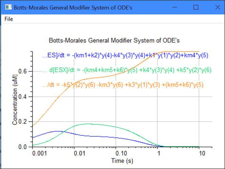
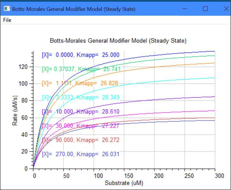
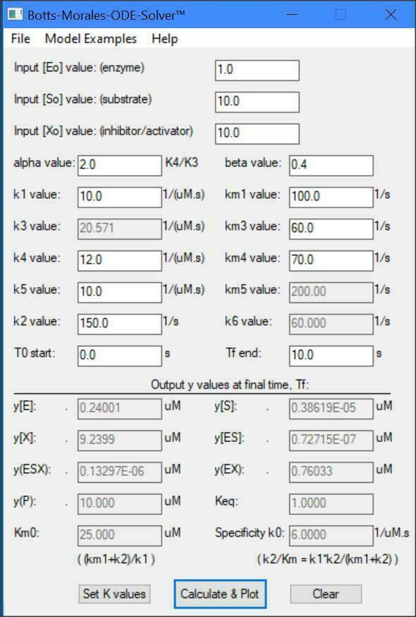
Botts-Morales General Modifier Models
K1 k2
E + S <===> ES ------> E + P
/\......................./\
K3 ||......................|| K4
\/.......................\/
EX + S <===> ESX ------> EX + P
K5 k6
Dissociation constants: K1 = km1/k1, K5 = km5/k5
Dissociation constants: K3 = km3/k3, K4 = km4/k4
k2 = kcat1, k6 = kcat2, Km = (km1 + k2)/k1
E = [Enzyme], S = [Substrate], X = [Inhibitor/Activator]
The letter ''m'' = minus = reverse direction (e.g., km1)
y(1) = dE/dt = -k1[E][S] -k3[E][X] +km3[EX] +(km1+k2)[ES]
y(2) = dS/dt = -k1[E][S] -k5[EX][S] +km1[ES] +km5[ESX]
y(3) = dX/dt = -k3[E][X] -k4[ES][X] +km3[EX] +km4[ESX]
y(4) = dES/dt = -k4[ES][X] +k1[E][S] +km4[ESX] -k2[ES]
y(5) = dESX/dt = -km4[ESX] -km5[ESX] +k4[ES][X] +k5[EX][S] -k6[ESX]
y(6) = dEX/dt = -k5[EX][S] -km3[EX] +k3*[E][X] +(km5+K6)[ESX]
y(7) = dP/dt = +k2[ES] +k6[ESX]
Reference:
1-Botts,J. & Morales,M., Trans. Faraday Soc. 49, 697-707 (1953)
2-Ricard,J., Biochem. J. 175,779-791 (1978), Generalized Microscopic Reversibility, Kinetic Co-operativity of Enzymes and Evolution 3-Weber,G., Biochemistry 11:864–878 (1972), Ligand binding and internal equilibria in proteins.
4-Baici,A., Kinetics of Enzyme-Modifier Interactions, Chapter 2, The General Modifier Mechanism, Springer-Verlag Wien (2015).
Your cart is empty
0
item(s)
/
$0
Checkout
Clear cart